Predictive Analytics: An Introductory Overview

What is Predictive Analytics?

Predictive analytics involves developing statistical models that predict an outcome or the probability of an outcome. For example, models can be developed to predict the income of customers or the probability of someone buying a particular product. These models are typically built using historical data or data collected specifically for the purpose of modeling. Predictive analytics is applied across various business and economic sectors, each demonstrating different levels of maturity. For instance, the financial services industry has used predictive analytics for many years, whereas areas like sports and retail are still evolving their use. Nevertheless, virtually every sector recognizes its importance for day-to-day decision making in both business and research.

Predictive Analytics Introduction

Standard Predictive Models

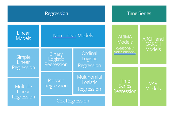
There are many standard predictive models that a data scientist should be familiar with. Some key examples include linear regression, logistic regression, Poisson regression, and time series analysis. As a data scientist, it is important to know which model to use in a given situation.

Below is a quick snippet of Python code illustrating a basic linear regression model on a small dataset. This code demonstrates how you might use a standard predictive approach to interpret data and predict outcomes:

import pandas as pd
from sklearn.linear_model import LinearRegression

# Sample dataset
data = {
    'Hours_Studied': [1, 2, 3, 4, 5],
    'Score': [20, 40, 50, 70, 80]
}

df = pd.DataFrame(data)

X = df[['Hours_Studied']]
y = df['Score']

# Fit a linear regression model
model = LinearRegression()
model.fit(X, y)

print("Intercept:", model.intercept_)
print("Coefficient:", model.coef_)

# Output:

Intercept: 6.999999999999993

Coefficient: [15.]

The graphic below summarizes the range of predictive models used in data science and analytics.

Predictive Modelling – A General Approach

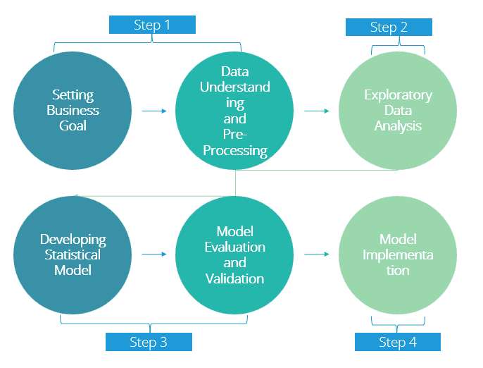
A general approach to building a predictive model often follows these steps:

1. Set a business goal or research objective.

2. Understand your data and carry out data pre-processing.

3. Perform exploratory data analysis (EDA).

4. Build and select the model, then validate it.

5. Implement the final model in a real-world environment.

Although this approach can vary depending on the problem and situation, these broad steps are common in predictive modelling.

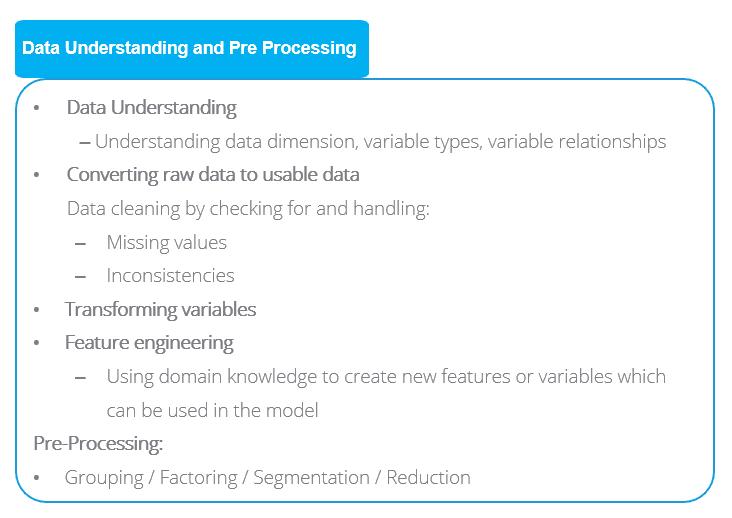
Data Understanding and Pre-Processing

The first step in predictive modelling is data understanding and pre-processing. Data understanding includes examining the dimensions of the dataset, variable types, and relationships between variables. Pre-processing might involve cleaning the data, handling missing values, removing inconsistencies, or transforming variables.

Feature engineering is another key component. Using domain knowledge, you can create new variables or transform existing ones in ways that make them more useful for modelling. In addition, you might group or factor variables to segment the data or reduce its dimensionality. Data pre-processing is critical and often consumes a considerable amount of time before actual model building begins.

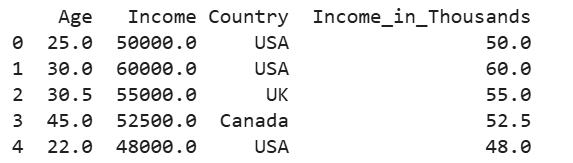
Here’s a quick example showing how you might handle missing values and transform a feature in Python:

import pandas as pd
import numpy as np

# Sample dataset with missing values
data = {
    'Age': [25, 30, np.nan, 45, 22],
    'Income': [50000, 60000, 55000, np.nan, 48000],
    'Country': ['USA', 'USA', 'UK', 'Canada', 'USA']
}

df = pd.DataFrame(data)

# Handling missing values by imputation
df['Age'].fillna(df['Age'].mean(), inplace=True)
df['Income'].fillna(df['Income'].median(), inplace=True)

# Creating a new feature based on domain knowledge
df['Income_in_Thousands'] = df['Income'] / 1000

print(df)

# Output:

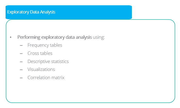
Exploratory Data Analysis

Once the data is ready, the next step is exploratory data analysis (EDA). During EDA, you typically generate descriptive statistics, create visualizations, and conduct correlation analysis to uncover patterns and relationships. This can help you decide which variables might be most relevant or whether some variables should be excluded altogether. EDA also yields valuable insights that strengthen your understanding of the dataset and inform subsequent predictive modelling decisions.

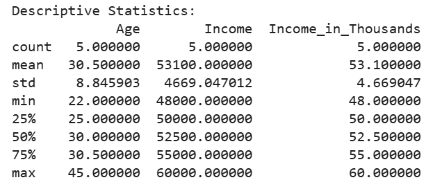
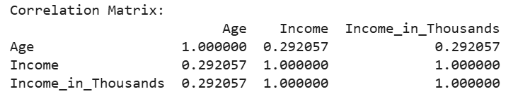
Below is an example of generating a correlation matrix and some basic descriptive statistics:

import pandas as pd

# Continuing from the previous df
print("Descriptive Statistics:")
print(df.describe())

# Output:

df1 = df[["Age","Income","Income_in_Thousands"]]
print("Correlation Matrix:")
print(df1.corr())

# Output:

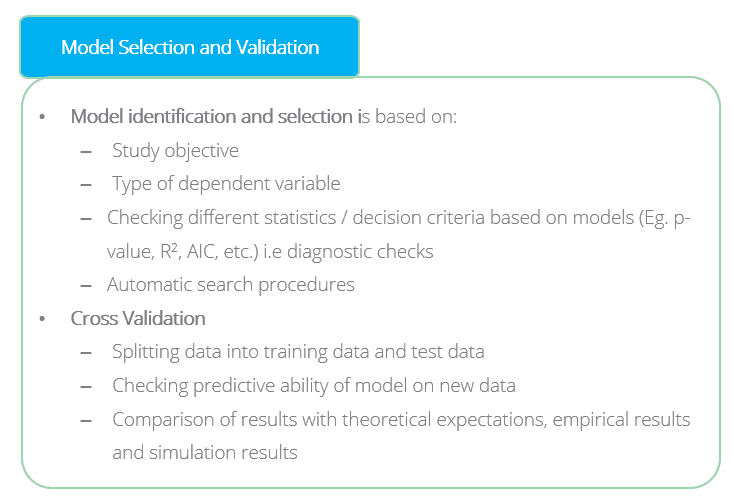
Model Identification, Selection, and Validation

The third step is identifying, selecting, and validating the model. Model identification depends on the type of dependent variable (continuous, binary, count, etc.). Based on the variable type, you would choose an appropriate method—such as linear regression for continuous variables or logistic regression for binary variables.

Model selection typically involves criteria like R-squared, p-values, or AIC. Additionally, automated search or model selection procedures (like stepwise selection) can be used. After the best-fitting model is chosen, you validate it using techniques such as cross-validation. This involves splitting the data into training and test sets, building the model on the training set, and using the test set to evaluate predictive performance. A successful performance on unseen data increases confidence that the model can be reliably implemented in a real-world setting.

For instance, here’s an example of splitting data into training and test sets:

from sklearn.model_selection import train_test_split
from sklearn.linear_model import LogisticRegression
from sklearn.metrics import accuracy_score

# Example dataset
data = {
    'Feature1': [2, 3, 5, 7, 9, 11],
    'Feature2': [1, 0, 1, 0, 1, 0],
    'Label':    [0, 1, 1, 0, 1, 0]
}

df2 = pd.DataFrame(data)
X = df2[['Feature1', 'Feature2']]
y = df2['Label']

# Split the data
X_train, X_test, y_train, y_test = train_test_split(X, y, test_size=0.3, random_state=42)

# Train a logistic regression model
log_model = LogisticRegression()
log_model.fit(X_train, y_train)

# Validate the model
predictions = log_model.predict(X_test)
print("Accuracy:", accuracy_score(y_test, predictions))

# Output:

Predictive Model Implementation

Finally, once a model is validated, it is ready to be implemented. Implementation can be as simple as deploying the model equation in a spreadsheet for analysts to use or as complex as integrating it into a large-scale IT system. It might also involve creating a standalone web application that provides a user-friendly interface for business users or a back-end service that automatically scores new data in real-time.

Sample Size and Data Dimension

Predictive models rely on historical or collected data. If the sample size is too small, the model might not accurately capture variable relationships. Conversely, if you have many variables but only a small number of observations, the model can become unstable or overfitted. A rule of thumb suggests having at least 10 observations for each variable. For instance, if you have 8 variables, you’d want at least 80 observations.

Recap

In this blog, we introduced predictive analytics and highlighted several areas where it’s applied. We also outlined a four-step general approach to model building:

1. Data understanding and pre-processing

2. Exploratory data analysis

3. Model identification, selection, and validation

4. Model implementation

Understanding these core steps and the corresponding techniques is essential for successfully applying predictive analytics to real-world business or research problems.