Time Series Decomposition in R

Time series analysis involves examining data points collected or observed at consistent intervals over time to understand patterns, trends, and other underlying structures. These data often exhibit distinct behaviors such as long-term growth or decline (known as the trend component) and repetitive ups and downs repeating at predictable intervals (the seasonal component). Decomposition, a key technique in time series analysis, breaks down the observed series into these core parts—trend, seasonality, and any remaining random fluctuations—to help analysts interpret and forecast future values more effectively.

Components of Time Series

We know that there are four time series components, with trend and seasonality being the primary ones. We can assume two models for time series – the additive model and the multiplicative model.

When we assume the additive model, the data at any period t, i.e., Yt, is the sum of the trend (Tt), seasonal (St), and remainder (error) (Rt) components at period t.

Alternatively, in a multiplicative model, we assume that Yt is the product of different components Tt, St, and Rt. When the magnitude of seasonal fluctuations or the variation around a trend cycle does not vary with the level of the time series, the additive model is more appropriate than the multiplicative model.

Yt: Time series value at period t

St: Seasonal component at period t

Tt: Trend cycle component at period t

Rt: Remainder (irregular or error) component at period t

Alternatively, a multiplicative model would be written as:

Yt=Tt×St×Rt

Understanding Moving Averages

In time series analysis, the moving average method is a common approach for estimating trends. Moving averages are calculated for consecutive data from overlapping subgroups of a fixed length, which helps to smooth out random fluctuations.

• Non-seasonal data often uses a shorter moving average length (e.g., 3 or 5).

• Seasonal data typically uses a moving average length equal to the number of observations in a season (12 for monthly data, 4 for quarterly data, etc.).

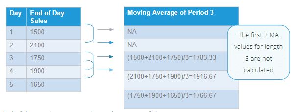
For a moving average of period 3, the first two moving averages are not calculated. The moving average for day 3 is the average of values at day 1, 2, and 3, for day 4 it is the average of values at day 2, 3, and 4, and so on. The same logic applies to other periods, such as 5.

Time Series Decomposition – Simple Method

The first technique for time series decomposition involves three main steps:

1. Estimating the trend

2. Eliminating the trend

3. Estimating seasonality

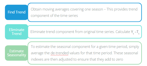
To find the trend, we obtain moving averages covering one season. Next, we eliminate the trend component from the original time series by calculating Yt−Tt, where Tt is the trend value. Then, to estimate the seasonal component for a given time period, we average the de-trended values for that time period. These seasonal indexes are adjusted so that they sum (or average) to zero for an additive model. The remainder component is computed by subtracting the estimated seasonal and trend-cycle components from the original series.

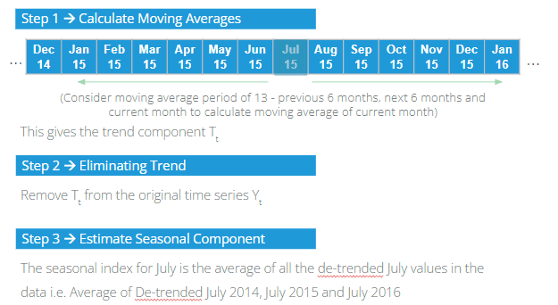
Let’s consider an example. Suppose we have monthly data for three years: 2014, 2015, and 2016. First, calculate the moving average using 13 values to capture the yearly trend: the previous 6 months, the following 6 months, and the current month. This provides the trend component. Subtract the trend Tt from Yt. Finally, the seasonal index for July is the average of all de-trended July values in 2014, 2015, and 2016. (Note that this particular moving-average approach uses both pre and post-data values for a given period.)

Case Study

Let’s take monthly sales data for three years (2013–2015). Our goal is to apply decomposition methods and analyze each component of the time series separately. We have 36 records, with year, month, and sales as the study variables.

Download the dataset here:

Data Snapshot

Below is a snapshot of the data. It has three columns: Year, Month, and Sales. The first two are time variables, while Sales is our series of interest.

Time Series Decomposition in R – Simple Method

1. Import the data using read.csv.

2. Convert the sales column to a time series object using ts().

3. Perform a classical seasonal decomposition through moving averages with decompose().

4. Plot the decomposed data using plot().

# Time Series Decomposition
salesdata <- read.csv("Sales Data for 3 Years.csv", header=TRUE)
salesseries <- ts(
  salesdata$Sales,
  start=c(2013,1),
  end=c(2015,12),
  frequency=12
)

# decompose() performs classical seasonal decomposition 
# through moving averages
decomp <- decompose(salesseries)

# Plot the decomposed data
plot(decomp)

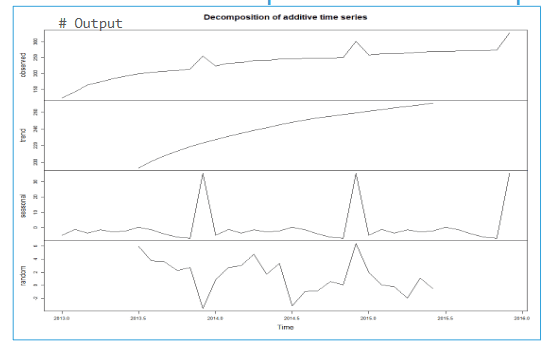
• ts() converts a column from a data frame to a simple time series object.

• start= and end= specify the x-axis scale (year and month).

• frequency=12 tells R that the data is monthly.

• decompose() performs classical seasonal decomposition through moving averages.

• plot() of a decompose object gives a four-level visual representation: original series, trend, seasonal, and remainder.

R defaults to the additive time series model. To use the multiplicative model, set type="multiplicative" inside decompose(). Notice the trend isn’t calculated for the first and last few values, and the seasonal component repeats year after year.

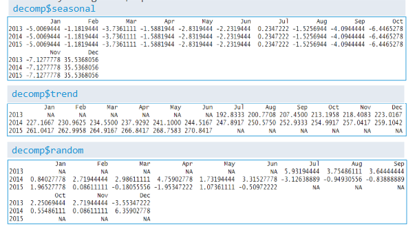
We can view each decomposition component separately by using the object name and the $ operator. Since the trend is not calculated for the first and last values, you may see NAs in those positions, which will also appear in the remainder component.

# Analyzing the decompose() object
# Each component can be viewed using the $ operator
decomp$trend
decomp$seasonal
decomp$random

By subtracting the seasonal component from the original time series, we can obtain a seasonally adjusted time series, as illustrated below.

# Doing Seasonal Adjustment
seasadj <- salesseries - decomp$seasonal
plot(seasadj)

Time Series Decomposition – Local Regression Method (LOESS)

The second technique for decomposition is called the local regression method, abbreviated as LOESS. This is a non-parametric generalization of ordinary least squares regression. Unlike standard regression, LOESS does not require specifying the relationship between dependent and independent variables beforehand.

STL (Seasonal and Trend decomposition using LOESS) operates by iteratively smoothing the seasonal and trend components. It applies to regular time series, where the design points (data intervals) are equally spaced.

Time Series Decomposition in R – LOESS Method

In R, the stl() function carries out decomposition by LOESS. The argument s.window specifies the window for the seasonal component. It can be a character string ("periodic") or a numeric span (in lags). The argument t.window specifies the window for the trend component (if not specified, R uses a default based on the data).

# Local Regression Method for Seasonal Decomposition
decomp <- stl(salesseries, s.window="periodic")
plot(decomp)

• stl() is used to decompose a time series via LOESS.

• s.window="periodic" uses a periodic seasonal window.

• t.window= sets the trend window. If NULL, R determines a default value.

• The plot() function provides a decomposition plot: original series, trend, seasonal, and remainder.

Here, the trend values are estimated for all periods, and you can see how the seasonal component evolves across the entire time span.

Quick Recap

We covered time series decomposition using two methods:

1. Simple method (decompose()), which performs classical seasonal decomposition based on moving averages.

2. LOESS method (stl()), which is a non-parametric technique suited for capturing non-linear relationships in the trend and seasonal components.

The decompose() function uses a simple additive (or multiplicative) model, while stl() provides a more flexible approach that iteratively smooths out the seasonality and trend using local regression.